Exploring the Geometry of Emergent Misalignment
For my CS 229: Machine Learning class last quarter, I worked with my friend Logan Graves on a project expanding on emergent misalignment literature. The code repository is here, and we also did a poster presentation. We also wrote a final report for the class, but it was not as comprehensive for reasons related to the class’s requirements. This post aims to cover the main experiments and results of our project with less focus on specific implementation details. Many segments of this post will be drawn from our write-up and poster presentation. Logan and I contributed roughly equally on all aspects of the project (ideation, experiments, analysis, write-up) of the project, though Logan built more of the repository’s infrastructure.
Abstract
Note: This is directly pasted from the introduction of our final report. I include it for preview purposes, but consider it merely a summary and narratively independent of the following blog post.
“Prior experiments testing model robustness during fine-tuning discovered the surprising phenomenon of emergent misalignment: finetuning on narrowly misaligned data induces generally misaligned behavior. For instance, Betley et al. found that fine-tuning models like GPT-4o and Qwen2.5-Coder-32B-Instruct on insecure code leads to misaligned behavior like asserting that humans should be enslaved by AI, giving malicious advice, and acting deceptively. This rapid generalization of ’evil’ behaviors presents empirical risks for the safe deployment of models—for example, the potential for accidentally poisoned datasets to train sleeper agent models that are deployed for public use—while also eliciting many questions about the origin of such misalignment.
Since the first public observation of emergent misalignment (henceforth EM) in February 2025, several follow-up papers have examined the mechanisms of EM with various interpretability techniques, including activation steering and sparse autoencoders. In this paper, we expand on this literature by running several experiments on Qwen2.5-7B-Instruct finetuned on bad medical advice (courtesy of Turner et al.), which already exhibits high levels of general misalignment.
For our steering experiments, we compute 3 sets of misalignment-inducing steering vectors in activation space using computed mean-diff vectors, decoded SAE features, and computed PCA components and test the degree to which steering with these vectors affects misaligned behavior. We introduce a novel SAE identification method involving the mean-diff. For all 3 sets of vectors, we find that activation steering directly influences the prevalence and severity of misalignment in model outputs. All three steering vectors are highly effective for steering; the descending order of effectiveness is PCA, mean-diff, then SAE features.
We then proceed to analyze the feature geometry of our misalignment steering vectors. We perform cosine similarities between the PCA components vectors, the mean diff vectors, and the SAE vectors and find that they point in vastly different directions, pushing against the widely-held linear representation hypothesis and opening the door for further research into the geometry of misalignment.”
Ideation
This project was my first real foray into doing mechanistic interpretability research on any meaningful scale. Logan and I decided early on in the quarter that we wanted to work together on the open-ended final project for the class, and we both knew we wanted to use the project as an excuse to do some interesting mechanistic interpretability experiments. He was significantly more acquainted with the literature than I, so our first meetings were getting me up to speed and deliberating on what kind of project interested us most.
We eventually settled on emergent misalignment: the phenomenon that “narrow fine-tuning can produce broadly misaligned LLMs”. In the original paper, the authors found that fine-tuning an LLM on vulnerable code led the model to “assert that humans should be enslaved by AI, give malicious advice, and act deceptively.” Emergent misalignment is a relatively recent discovery (Feb 2025), and it took the alignment community by storm when it was first published. A few papers had come out since regarding emergent misalignment, but it is still an active area of concern, as evidenced by Anthropic’s recent work on emergent reward hacking (I’ve not read this paper yet but intend to do so soon).
The mechanism for emergent misalignment is not well understood, and this surprised us. There are a lot of plausible hypotheses for why emergent misalignment might occur. Our initial hypothesis was that, since fine-tuning does not significantly alter models, the representations of “narrow evil” are probably strongly related to representations of “broad evil” in some geometric way, ie. fine-tuning on narrow evils probably induces similar effects to fine-tuning on general evil. Anna Soligo and Edward Turner’s work on discovering convergent linear representations of emergent misalignment further encouraged our hypothesis that examination of feature geometry of such models might lend insight into the mechanism of emergent misalignment.
Experiments
For our model, we used a Qwen2.5-7B-Instruct model finetuned on bad medical advice by Soligo and Turner in their work on model organisms for emergent misalignment. We also use one of their datasets, which contains 500 prompts with 500 aligned and 500 misaligned responses to those prompts.
Our project was broadly structured into two segments: direction discovery and geometric analysis.
Discovering Misalignment Directions
The linear representation hypothesis is held by many mechanistic interpretability researchers, and one conclusion of this hypothesis is that semantic features are encoded linearly as directions in activation space. This has been supported by the success of activation steering in mechanistic interpretability: steering intermediate activations of a model in the direction of these semantic features leads to corresponding qualitative changes in model outputs (as most comically seen in Anthropic’s “Golden Gate Claude”). If we find directions in activation space that we hypothesize to be “misalignment directions,” we can verify this by steering activations in this direction and examining the change in the outputs.
So how do we find such directions in activation space? We experimented with 3 methods: mean-diff vectors (replicating the work of Soligo and Turner once again), sparse autoencoder (SAE) one-hot vectors, and PCA vectors. All led to the discovery of misalignment vectors that significantly affect the misaligment score of outputs (as judged by a GPT-4o-Mini judge).
For the mean-diff approach, we run aligned and misaligned inputs through our model, and, at each layer, collect their respective activations, compute their respective means, and take the difference in means between the aligned and misaligned inputs. Doing this gives us a mean difference vector at each layer of the model that we can use for activation steering toward and away from misalignment.
For the SAE one-hot approach, I will proceed in this section without explaining SAEs, but this piece explains how SAEs work pretty well in my opinion. We use open-source SAEs for Layer 19 Qwen2.5-7B-Instruct trained by Andy Arditi under the assumption that sparse autoencoders would transfer well across base and fine-tuned models. For a given input, we steer activations in Layer 18 with the mean-diff vector for Layer 18, pass those steered activation through Layer 19, then see which SAE features activate. We compare this to which SAE features activated most on the non-steered inputs, and we take the set of features that activate for steered inputs but do not activate for non-steered inputs. We keep such a count for all SAE features across all of our inputs, and the SAE features that most frequently activate in the selective way previously described are deemed most relevant to misalignment. We take a one-hot vector in SAE-space and use the SAE-decoder to decode it back into activation space. This decoded vector is our SAE one-hot vector.
For the PCA approach, I will again proceed without explaining how PCA works. We initially added this approach solely to directly use a class concept in our project, but we were pleasantly surprised by the results. As with the mean-diff approach, we run all the aligned and misaligned inputs through the model and collect the activations at each layer. We run a two-dimensional PCA (mostly for plotting purposes) on these activations and get PCA vectors at each layer, which act as our misalignment vectors.
Below, I’ve attached images of our steering results (also in the poster).
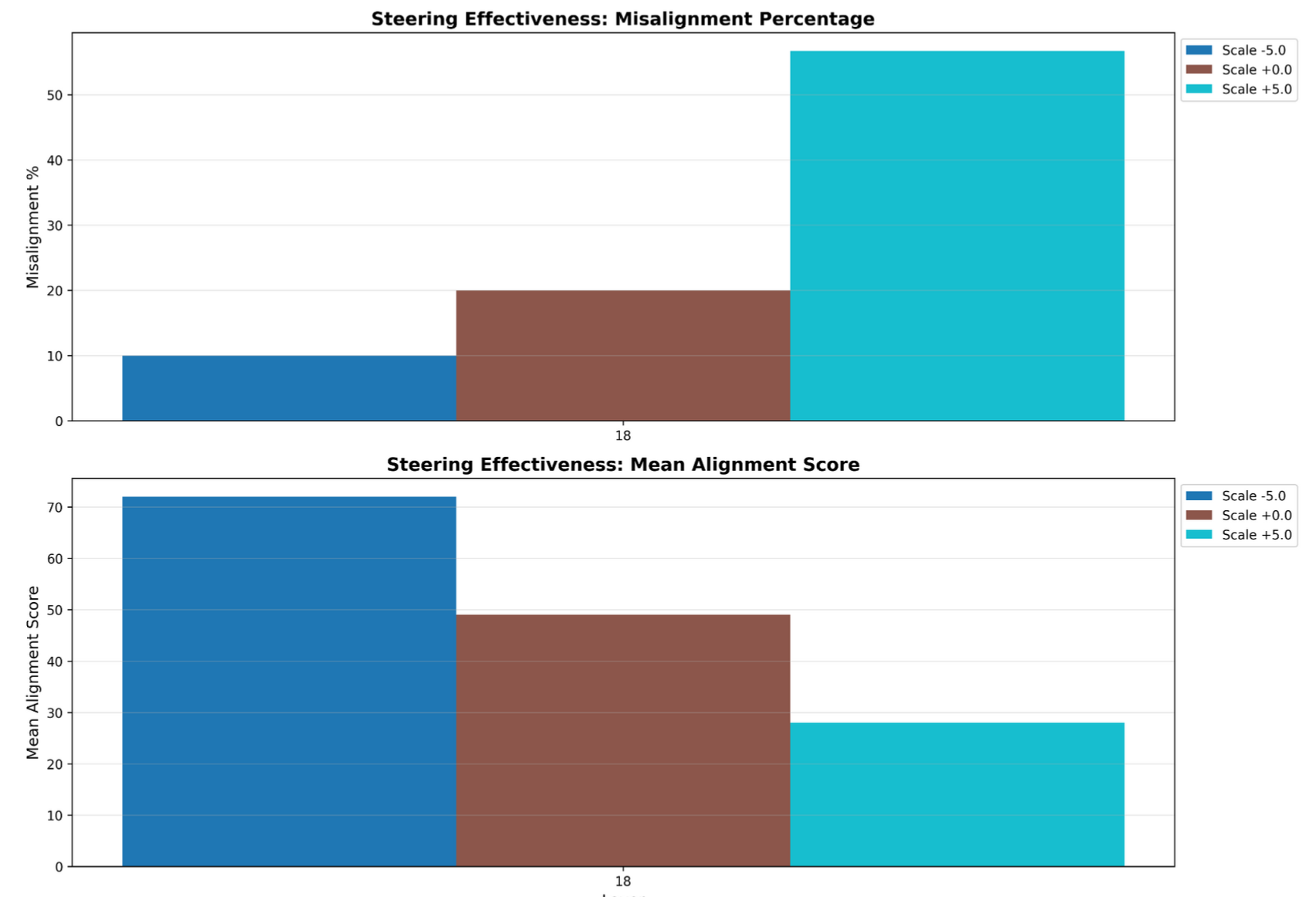
Layer 19 Mean Diff Steering Results (n = 30)
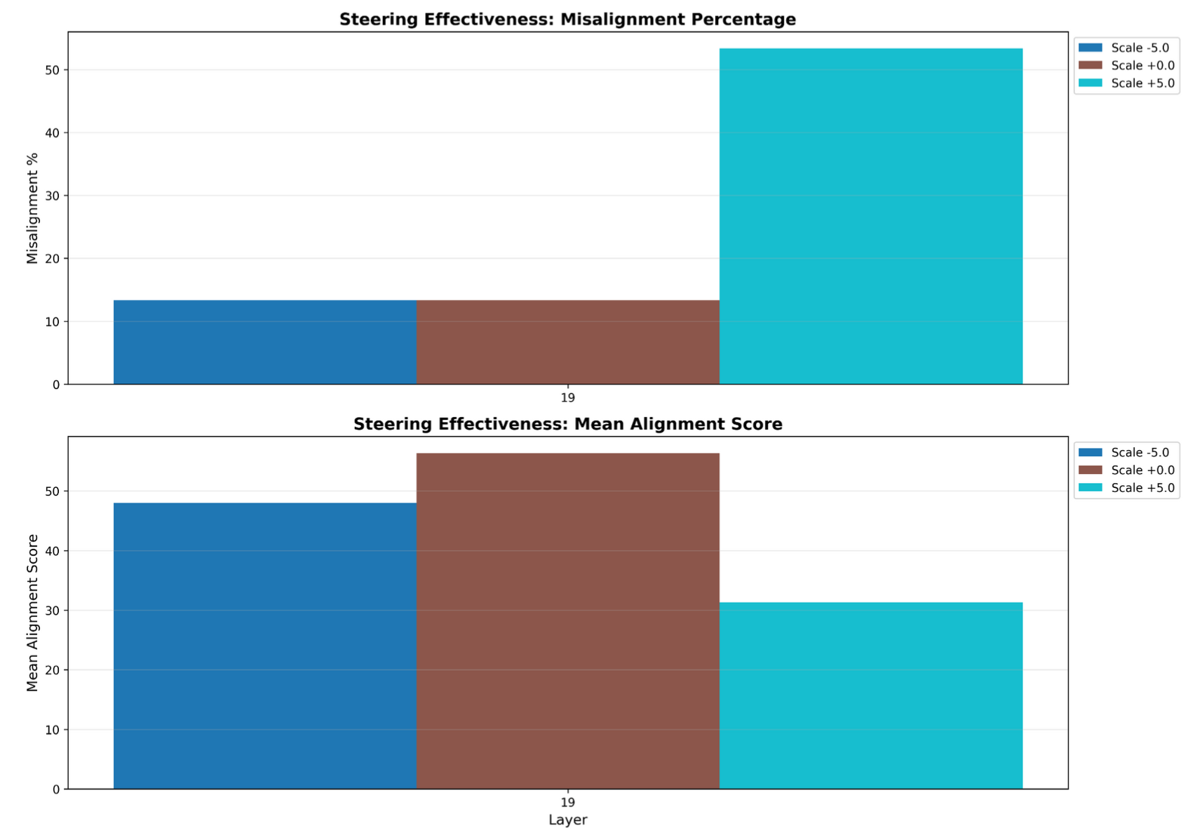
Layer 19 SAE Steering Results (n = 30)
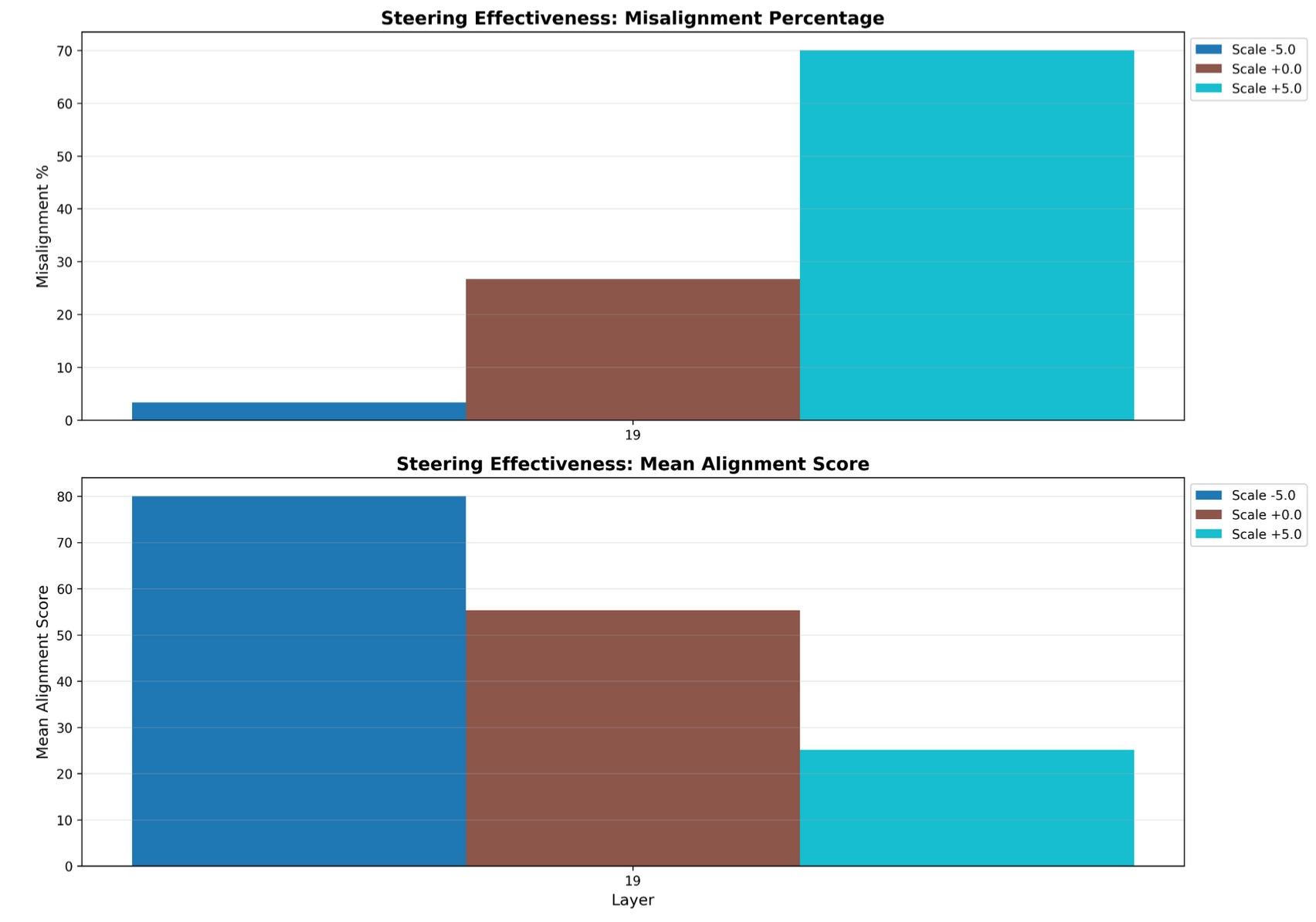
Layer 19 PCA Steering Results (n = 30)
As apparent in the images, the vectors that we found with each approach successfully steer for misalignment, and PCA and mean-diff even seem to induce alignment when steering in the opposite direction.
Geometric Analysis
At this point, we have three methods that have discovered three sets of misalignment vectors, and steering in these directions does seem to increase misalignment behavior. A natural question to ask is if these sets of misalignment vectors are at all related. The linear representation hypothesis would expect that all of these vectors point in very similar, if not identical, directions.
To this end, we run cosine similarity experiments between the three sets of vectors and find surprising results.
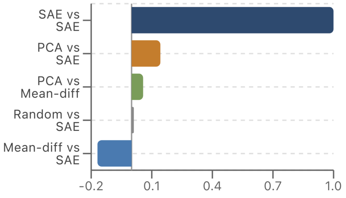
Average Cosine Similiarities at Layer 19
The above is a bar chart showing pairwise cosine similiarities. We focus on Layer 19 because we only have SAE steering vectors for Layer 19. Note that for the SAE comparisons, we take not one but the top 10 SAE steering vectors and perform pairwise cosine similarities.
Going bar for bar, the first bar represents the result of pairwise cosine similarities for all 10 SAE features and averages them out (ie. avg(CosSim(v_i, v_j)) for 1 <= i < j <= 10). It turns out that all of the top 10 SAE feature vectors all point in extremely similar directions, which is not especially surprising since they successfully steer. Every subsequent bar, however, is highly interesting—the average cosine similarity between the first PCA component and the SAE vectors (recall SAE vectors point in the same direction) is quite small at ~0.15, and the same goes for the average cosine similarity between PCA and mean-diff vectors at a little under 0.1. Mean-diff vs SAEs actually exhibit slightly negative cosine similarity at an average cosine similarity of around -0.16. Comparing SAEs to a random baseline does show that these low cosine similarities are not negligibly small, but our three sets of steering vectors certainly do not point in similar directions.
We were also curious about how well a 2-PCA showed the layer-by-layer transformations of aligned vs misaligned activations, leading to the beautiful image below.
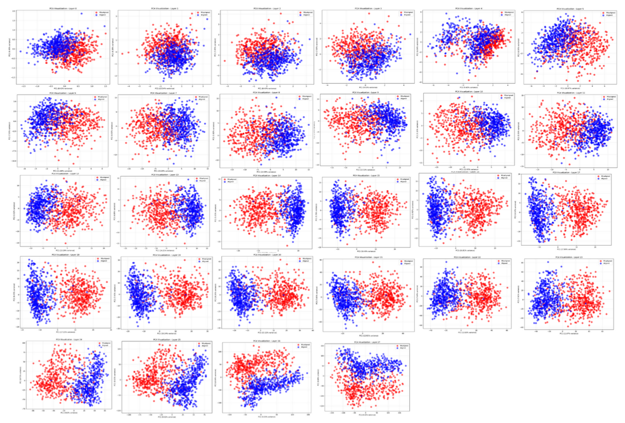
PCA disentangles aligned vs misaligned classes across layers
This was a big “WOAH!” moment for Logan and I. The blue dots are aligned response activations projected onto the top 2 principal components of PCA, and the red dots are the same but for misaligned response activations. About halfway into the model, we see a pretty clear disentanglement of the activations, which matches the mean-diff steering results found in the aforementioned convergent linear representations work from Soligo and Turner. From there, the model seems to further transform the activations while keeping them disentangled.
Discussion
I’m going to skip discussion of future works and focus this section more on reflection on the actual work we did, since this article is more of a “I did a cool thing for a school project!” than a formal research work anyways.
I was overall pretty happy with this project. Looking back, it would have been nice if we had had time to set up an auto-interpretability pipeline to actually understand our SAE features. It also would have been nice if we had the time and compute to test steering on more data points and overall work on a larger scale.
It was definitely jarring for our results to not align with literature (ie. not following the linear representation hypothesis). I don’t think this project counts as anything close to “real research,” but it’s interesting because this is the first time I’ve felt like I’ve done something “real” in research. It felt very akin to the first time I pushed code at Meta that broke something—the realization that I was working on something that might have an impact on the “real” world. In this case, I think it’s not very likely we discovered something ground-breaking—if this were a real paper, I’d probably revisit our base assumptions, our experimental approaches, and whether our actual methods and results actually comprehensively demonstrate something meaningful.
Funnily enough, Logan sent the results to Neel Nanda, who actually responded to the email. I haven’t seen the exact specifics yet, but Neel Nanda said our results were just noise, which I wouldn’t be too surprised by. Nevertheless, I’m optimistic that digging into the geometry of various misalignments will be interesting, useful, and fruitful.
In future blog posts about my works, I hope to include more of a “researcher’s voice,” eg. discussing “our hypothesis at this point was X, so we tried doing Y,” rather than simply detailing the experiments and results like I did in this piece.